When analyzing a system in fluid mechanics, we usually take one of two approaches: (1.) consider the flow of properties on a particle-based scale at every point in a given fluid (differential approach), or (2.) specify a fixed region and determine how its fluid properties vary with flow (control volume approach). Depending on your main interests, each approach offers its own advantages and disadvantages - along with different information. For example, consider diagram 1 which depicts a chamber containing two fluid inlets and one fluid outlet. Further, suppose you are interested in assessing how this device accumulates mass of a given chemical species. If you are a chemical engineer focused on production, you may concentrate on the flow of fluid properties inside the chamber - as opposed to how each individual particle flows. In that case, a control volume analysis would be more appropriate. The way in which fluid properties vary over the red, dotted region - which is fixed and formerly known as a control volume - would be of most interest. Conversely, if you are a researcher responsible for product development, you may be more interested in how the inlets/outlets affect flow and pressure distributions. In this scenario, the flow of individual particles as they enter/exit the chamber would offer more valuable information, and a differential approach becomes more appropriate. So, when studying fluid mechanics, keep in mind that each approach offers its own unique perspective and is tailored to specific situations.

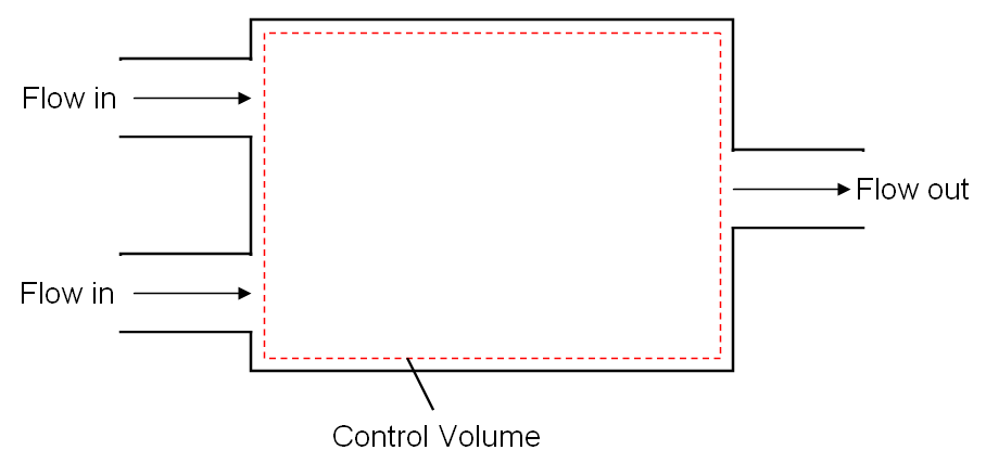
Diagram 1: Schematic of a mixing chamber used to demonstrate how different analytical approaches 1.) provide specific sets of information and 2.) lead to certain outcomes more efficiently than others.

     In this lesson, the goal is to first lay the foundations for a control volume approach - which is most commonly used in engineering studies and industrial applications. Such an approach will also be useful when developing the differential analysis in subsequent lessons. Before beginning, however, let's first recall how the most common conservation laws - such as conservation of mass, momentum, energy, etc - are used in solid mechanics. This will be useful for considering the flow of properties over our control volume and extending these laws to fluid mechanics. 

      When dealing with solid mechanics, conservation laws are developed over an entire system of particles. Such a system is defined by a fixed quantity of mass enclosed in distinct, fixed boundaries. For example, consider a rigid, cylindrical piece of aluminum. This solid body contains a fixed mass enclosed in a cylindrical region or boundary. 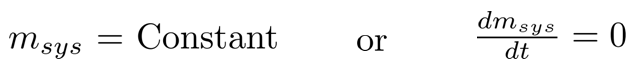To apply any conservation law to this rod, we would have to consider how properties are conserved over the entire system inside the specified boundaries. For instance, conservation of mass asserts that no mass is created or destroyed within the system's boundaries:

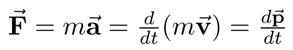
Similarly, conservation of momentum - which leads to Newton's familiar second law - dictates that any exterior forces exerted on the system's boundaries will incite motion:

In either case, the rigid body's system - along with its boundaries - is fixed as time progresses, and the system ultimately remains unchanged - even though it may move. In other words, the rigid bodies studied in solid mechanics generally possess a fixed volume and mass. This is very beneficial when applying conservation laws - since the volume of interest always coincides with the total mass.
    
     Conversely, when considering a fluid-based system, this is usually not the case; the system's boundaries can change with time as the fluid evolves. For example, if you have a bucket of water, that system will initially contain a specific amount of mass in a given volume. However, unlike the solid rod discussed above, turning that bucket upside down will change the system's volume, and the boundaries no longer remain constant. This makes the application of conservation laws a bit more complex and challenging. Unlike the equivalent case in solid mechanics, setting the volume of interest equivalent to that inside the system's boundaries is no longer practical. Not only would this volume continually change in an unpredictable manner, but we are generally interested in conservation laws over a given, fixed region. For instance, in the example used for diagram 1, the chemical engineer was interested in the flow of properties inside the mixing chamber - not within the system's changing boundaries. This is where the control volume approach comes into play and addresses this dilemma. By focusing on a fixed region, the control volume approach allows us to once again analyze a volume with definite boundaries - as is done in solid mechanics. However, since the conservation laws apply to a system, the main challenge resides in translating these system-based laws over to a control volume basis. This is accomplished using the Reynolds Transport Theorem (RTT) - the derivation of which forms the basis of this lesson.

     As mentioned in the previous section, the lesson's main goal is to reformulate system-based conservation laws such that they may be applied over a fixed, control volume. This will be accomplished by first considering a simplified, straightforward example - one-dimensional duct flow. Then, after establishing the basic concept, the new conservation law will be extended to a generalized case. Focusing first on the simplified case, suppose that fluid is flowing through a rectangular duct with one-dimensional flow. In other words, the velocity only changes along the duct's length in the x-direction (V = V(x)); no change is observed along the y- and z-directions. Depicted in Diagram 2, the fluid originally contains three separate systems (I, II, and III) at an initial time t. Furthermore, the selected control volume - which is depicted in red and lies between points a and b - originally encloses all of system II, and systems I and III initially reside outside of the control volume. Now, as time progresses, you can imagine that all three systems will flow to the right, and system II will begin to leave the fixed control volume. Similarly, system I will also begin to enter the control volume. This is shown in Diagram 2 (b.) for a time t + dt - where dt is a small, incremental change in time. You can clearly see that system I has entered the control volume (signified by the green region), while a portion of system II has left (represented by the orange area). What we are really concerned with though is not how the separate systems evolve. Rather, we want to know how fluid properties change in the control volume's fixed region and how that relates to a given system.

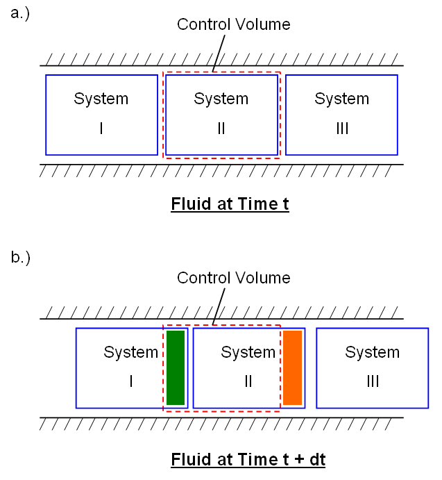
Diagram 2: Sketches of the simplified example broken down into three separate systems. At time t when the analysis begins (sketch a), the specified control volume initially coincides with System II. However, as time progresses by an amount dt (sketch b), a portion of this system leaves the control volume - while a fraction of System I enters.

     To do this, we must first distinguish between extensive and intensive fluid properties. Traditionally, extensive properties are those which are contingent on the extent - or overall size - of a given system. Typical examples of extensive properties are energy, mass, and momentum - quantities proportional to a system's total amount of matter. For example, if you take a bucket of water, dumping half of the contents into two separate buckets will change the extensive properties. The two new buckets will end up with half of the original bucket's total mass and energy. Conversely, intensive properties are independent of a given system's size; they are inherent bulk properties describing the entire system - regardless of its total amount of matter. Common examples of intensive properties are density and temperature; knowledge of the entire system is not needed to define each quantity. Working with the previous example above, the water density and temperature found in both the initial and two subsequent buckets would most likely be equivalent. Changing the system's size (or extent) has no effect upon the overall property. Before moving on, it is important to quickly note a special subset of intensive properties: specific properties. These properties are identical to intensive properties but are defined on a per-mass basis. Some common examples include specific volume (m3/kg), enthalpy (kJ/kg), and internal energy (kJ/kg). As will be shown shortly, this subset of properties is particularly useful for computing a given region's extensive properties.

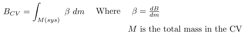
     Now, suppose that you are interested in some extensive fluid property B (mass, momentum, energy, etc), which has a corresponding intensive property β. In this case, we will take that intensive property to also be a specific property; so, β then represents the total amount of B per unit mass of fluid (or β = dB/dm). To calculate the total amount of B in a given region (such as the control volume in Diagram 2), we can take its respective intensive property β and simply integrate over the region of interest. This is why knowledge of a system's intensive property becomes so important; it allows us to quickly calculate its cumulative extensive property with minimal effort. For any given control volume, this process is expressed mathematically as follows:

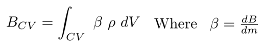
If the density is constant throughout a given region, this expression may also be further simplified. To do so, we will express each infinitesimal element of mass dm as a function of the fluid density ρ and element volume dV. This yields the following result - which is much easier to evaluate for a given control volume: 

Using this expression, we can then evaluate the total amount of any extensive fluid property found in a given region. It is also important to note that the constant density assumption employed above is quite reasonable. While not always the case, the majority of fluids are incompressible - especially water and other liquids; this means that density remains fairly constant, as the applied pressure increases. So, regardless of the fluid's state, it is reasonable to assert that density remains constant for all times t and throughout the domain.

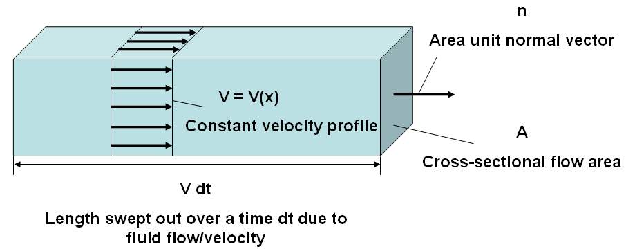
Diagram 3: As the fluid flows through this example's duct, it will sweep out a volume whose length is V dt, and the cross-sectional area A will remain constant; such a volume is depicted above. Thus, we may compute this sweeped volume as the product of that length and constant area (ie Volume = V A dt). Using the extensive/intensive property framework established above, this volume term can then be utilized to determine the total extensive property B flowing in or out of the control volume (or, in other words, the flux terms).

     Returning to the simplified example above, we can now define the total amount of any extensive property B in the specified control volume. However, as explained above, fluid flow will also carry some properties into and out of the control volume (refer to the green and orange regions in Diagram 2 b.), respectively). Thus, in order to eventually perform a balance, we will need to mathematically describe this process; so, let's do that now. 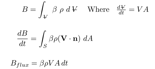Fortunately, in this simplified example, we have made two important assumptions which greatly simplify the calculations. As the fluid flows through the duct, the cross-sectional area remains constant, and there is no cross-sectional variation in the velocity profile (ie V = V(x)). This allows us to express each flux term using constant values and sidestep any surface integrals. Under these assumptions for a given time dt, the total volume swept through a constant area A is then equivalent to that of a rectangular prism. Such a prism has a total sweep length of (V dt) and encloses the volume depicted in Diagram 3. Using this volume, we may then define the fluid property B flowing in or out of the control volume as follows; this uses the same exact framework laid out above for BCV:

     At this point, we now have all essential ingredients for considering the change of extensive property B over the control volume. Remember, though; we are certainly interested in how fluid properties change over a given control volume, but the main goal is to relate that to changes in a given system. This will be accomplished by considering a fluid property balance over Diagram 2's control volume. As shown in Diagram 2 a.), it is clear that system II initially coincides with the control volume. So, at reference time t, we will assert that BCV (t) = BsysII(t) and explore how this relation varies with time. After an incremental time dt has passed, we already know that fluid flows into and out of the control volume; this is captured by the green and orange areas in Diagram 2 b.), respectively. Hence, after a time dt has passed, a portion of system II has flown out of the control volume, while other fluid has entered. So, the extensive property B at time t + dt may be expressed as BCV(t + dt) = BsysII(t + dt) - Bflux, out + Bflux, in (refer to Diagram 2 (b.); I am simply adding up the separate regions). Using this information, we can then approximate the control volume's change of extensive property B as follows:

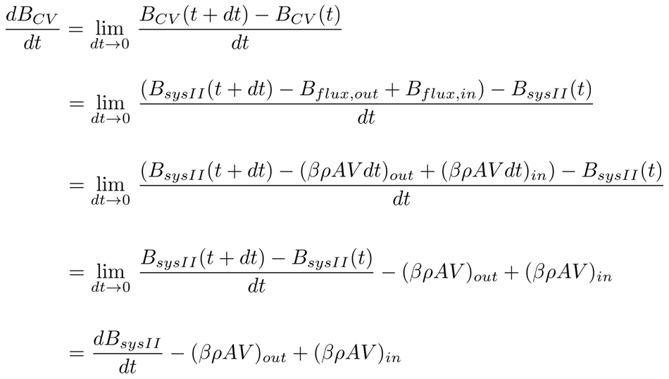
In the last line above, I used the limit-based definition of a derivative to express system II's rate of change. At this point, we now have an expression relating changes between the control volume and system. However, as explained above, the conservation laws are expressed on a system-basis; so, let's solve for the system term and make a few finishing touches:

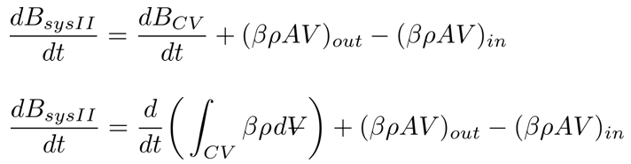
Using this expression, we now not only know how an extensive property B changes in a given system, but this also allows us to apply the common conservation laws - such as conservation of mass, momentum, energy, etc - to a specified control volume. This will be accomplished in subsequent lessons and play a huge role in extending physical models to fluid mechanics.

Like our content? Share it with your friends!

Or join the discussions on our community forum!


Leave a comment     Start a new thread